Divide and conquer

Divide and conquer is an algorithm design paradigm in which a problem is divided into smaller subproblems (often two ones) of the same type and then each subproblem is solved independently. The division is applied recursively until sub-problems become simple enough to be solved directly using a base case. Finally, the solutions of all sub-problems are combined to get the solution for the original problem. Let’s consider each of the described steps in more detail.

The steps of a divide and conquer based algorithm

A typical algorithm based on the divide and conquer paradigm consists of three steps:

1. Divide: split a problem into smaller sub-problems of the same type. Each sub-problem should represent a part of the original problem.
2. Conquer: recursively solve the sub-problems. If they are simple enough, solve them directly using base case conditions.
3. Combine: unite the solutions of the sub-problems to get the solution for the original problem.

The following picture shows the steps and their results:

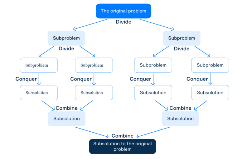
In the above example, we first divide the original problem into two subproblems. Each subproblem is then divided into new subproblems until they are small enough to be solved directly. After solving the smallest subproblem, we obtain subsolutions. Then, the subsolutions are combined to get subsolutions for more complex subproblems. The process continues until we obtain the solution for the original problem. As you can see, the presented process is recursive by its nature.

A simple example: the sum of elements in an array

Let’s consider how the divide and conquer paradigm can be used to calculate the sum of elements in an array. Note that the problem can be solved more efficiently and in a more simple way. Here, we apply the paradigm just to get a better understanding of how it works. The procedure is the following:

calc_sum(array, left, right):
    # the sum of zero elements is 0
    if left == right:
        return 0    
 
    # the sum of one-element sub-array is the element
    if left == right - 1:
        return array[left]
 
    # the index of the middle element to divide the array into two sub-arrays
    middle = (left + right) / 2;
 
    # the sum of elements in the left subarray
    left_sum = calc_sum(array, left, middle)
 
    # the sum of elements in the right subarray
    right_sum = calc_sum(array, middle, right)
 
    # the sum of elements in the array
    return left_sum + right_sum

The method takes an array of numbers and two variables named left and right. The variables correspond to the boundaries of a subarray where the sum should be calculated. The left boundary is inclusive, the right is exclusive.

The first two if conditions of the method correspond to base cases: they don’t perform a recursive call but immediately return a result. The next statement corresponds to the divide step: we calculate the middle element thus dividing the array into two subarrays. The next two statements represent the conquer step: we calculate the sum for each subarray. Finally, we unite the sums together and return it as a final result.

Below you can see several examples of how the procedure works for different arrays:

single_elem_arr = [55]
sum1 = calc_sum(single_elem_arr, 0, 1) # 55
 
two_elems_arr = [14, 36]
sum2 = calc_sum(two_elems_array, 0, 2) # 50
 
five_elems_arr = [14, 27, 31, 54, 38]
sum3 = calc_sum(five_elems_arr, 0, 5) # 164

Examples of divide and conquer based algorithms

There are many widely-used and efficient algorithms based on the divide and conquer paradigm: binary search, merge sort, quick sort, and others. We will learn these algorithms in the following topics and will see how the paradigm works for each of them.